muvis
muvis is a visualization and analysis toolkit for multivariate datasets. To use this package, you will need the R statistical computing environment (version 3.0 or later).
Installation and import
muvis can be installed through github:
# To set BioC as a repo
setRepositories(ind = c(1, 2))
devtools::install_github("bAIo-lab/muvis")
library(muvis)
NHANES Dataset
Dateset
The National Health and Nutrition Examination Surveys (NHANES) is a program of studies about health and nutrition for US residents. We examined the functionality of muvis on NHANES 2005-2006 dataset which contains 7449 variables and 10,348 samples. For more details about variable names and samples visit website- https://www.icpsr.umich.edu/icpsrweb/ICPSR/studies/25504/summary
Based on the number of missing values, we selected 161 variables including one ID, 74 continuous, and 86 categorical variables (having two to fifteen levels) and 4461 individuals (samples) aged from 20 to 85 years, including about 1% missing values. Complete list of 161 variables is available in NHANES dataset of the package.
data("NHANES")
# Set ID variable to NULL
NHANES$SEQN <- NULL
data_preproc
We use data_preproc function with levels = 15 for preprocessing (imputing missing values and specifying categorical and continuous variables) of NHANES. The detect.outliers option is used to exclude outliers for each variable.
data <- data_preproc(NHANES, levels = 15, detect.outliers = T, alpha = .5)
kableExtra::kable(head(data)) %>%
  kable_styling() %>%
scroll_box(width = "100%", height = "200px")| BMXWT | BMXHT | BMXBMI | BMXLEG | BMXARML | BMXARMC | BMXWAIST | BMXTHICR | RIDAGEYR | DBD091 | LBXIGE | LBXBCD | LBXBPB | LBXWBCSI | LBXLYPCT | LBXMOPCT | LBXNEPCT | LBXEOPCT | LBXBAPCT | LBXRBCSI | LBXHGB | LBXHCT | LBXRDW | LBXPLTSI | LBXCRP | LBXRBF | LBXFOL | LBXGH | LBDHDD | LBXHCY | LBXPT21 | LBXCOT | LBXSAL | LBXSATSI | LBXSASSI | LBXSAPSI | LBXSBU | LBXSCA | LBXSCH | LBXSC3SI | LBXSCR | LBXSGTSI | LBXSGL | LBXSIR | LBXSLDSI | LBXSPH | LBXSTB | LBXSTP | LBXSTR | LBXSUA | LBXSNASI | LBXSKSI | LBXSCLSI | LBXSOSSI | LBXSGB | LBXTC | LBXTHG | URXUMA | URXUCR | LBXALC | LBXBEC | LBXCRY | LBXGTC | LBXLUZ | LBXLYC | LBXVIA | LBXVIE | LBDTLY | LBXB12 | LBXVIC | LBXVID | PEASCTM1 | BPXSY | BPXDI | RIAGENDR | RIDRETH1 | INDHHINC | AGQ010 | AGQ040 | AGQ100 | AGQ120 | AGQ180 | AUQ131 | BPQ020 | HSD010 | DPQ010 | DPQ020 | DPQ030 | DPQ040 | DPQ050 | DPQ060 | DPQ070 | DPQ080 | DPQ090 | DBQ197 | DSD010 | DSD010AN | DIQ010 | DIQ190A | DIQ190B | DIQ190C | DIQ200A | DIQ200B | DIQ200C | FSD032A | FSD032B | FSD032C | HIQ011 | HUQ010 | HUQ020 | HUQ030 | HUQ050 | HOQ011 | HOQ040 | HOD060 | HOQ065 | HOQ230 | HOQ240 | IMQ011 | KIQ022 | MCQ010 | MCQ080 | MCQ140 | OHQ011 | OHQ620 | PAD020 | PAQ100 | PAQ180 | PAD200 | PAD320 | PAD440 | PAQ500 | PAQ520 | PAD590 | PAD600 | RDQ070 | RDQ140 | SLD010H | SLQ030 | SLQ050 | SLQ060 | SLQ090 | SLQ100 | SLQ110 | SLQ140 | SLQ170 | SLQ200 | SLQ210 | SMD410 | VIQ031 | LBXHA | LBXHBC | LBDHBG | LBXHBS | LBDHCV | BPXPULS | DBQ095Z | DRQSPREP | DRQSDIET | DRD360 |
|---|---|---|---|---|---|---|---|---|---|---|---|---|---|---|---|---|---|---|---|---|---|---|---|---|---|---|---|---|---|---|---|---|---|---|---|---|---|---|---|---|---|---|---|---|---|---|---|---|---|---|---|---|---|---|---|---|---|---|---|---|---|---|---|---|---|---|---|---|---|---|---|---|---|---|---|---|---|---|---|---|---|---|---|---|---|---|---|---|---|---|---|---|---|---|---|---|---|---|---|---|---|---|---|---|---|---|---|---|---|---|---|---|---|---|---|---|---|---|---|---|---|---|---|---|---|---|---|---|---|---|---|---|---|---|---|---|---|---|---|---|---|---|---|---|---|---|---|---|---|---|---|---|---|---|---|---|---|---|---|
| 75.2 | 156.0 | 30.90 | 38.0 | 35.0 | 35.8 | 96.0 | 53.7 | 44 | 1.0000 | 29.80 | 0.14 | 1.01 | 5.300000 | 35.80000 | 7.8 | 55.1 | 0.9 | 0.5 | 4.63 | 12.5 | 37.1 | 13.7 | 298 | 0.2848381 | 272 | 9.8000 | 6.000000 | 39 | 9.330000 | 80.00000 | 0.035 | 3.5 | 14 | 16 | 74.00000 | 6 | 8.9 | 103 | 23 | 0.8 | 17 | 87.00000 | 51 | 105 | 3.4 | 0.4 | 6.9 | 78 | 4.9 | 137 | 4.1 | 106 | 271 | 3.4 | 105 | 1.97 | 18.00000 | 202 | 1.300000 | 5.30000 | 2.500000 | 135 | 8.7 | 11.0 | 41.7 | 604 | 23.6 | 510 | 0.82 | 12 | 827.0000 | 139.3333 | 73.33333 | 2 | 4 | 3 | 2 | 2 | 2 | 2 | 2 | 2 | 1 | 3 | 1 | 1 | 1 | 1 | 1 | 1 | 1 | 1 | 1 | 2 | 2 | 2 | 2 | 2 | 2 | 2 | 2 | 2 | 2 | 3 | 3 | 3 | 1 | 3 | 1 | 1 | 6 | 2 | 3 | 4 | 1 | 2 | 2 | 3 | 2 | 2 | 2 | 2 | 4 | 3 | 1 | 1 | 1 | 2 | 2 | 2 | 2 | 3 | 3 | 1 | 2 | 2 | 12 | 2 | 2 | 2 | 1 | 1 | 1 | 1 | 2 | 2 | 2 | 2 | 2 | 2 | 2 | 2 | 2 | 2 | 1 | 4 | 3 | 2 | 1 |
| 69.5 | 167.6 | 24.74 | 40.4 | 37.5 | 31.2 | 96.5 | 48.0 | 70 | 1.0000 | 17.40 | 0.14 | 1.86 | 7.500000 | 29.40000 | 9.1 | 58.9 | 2.2 | 0.4 | 4.72 | 14.5 | 42.6 | 12.5 | 225 | 0.0500000 | 373 | 18.7000 | 5.353824 | 59 | 8.960000 | 44.00000 | 0.021 | 5.0 | 31 | 29 | 48.00000 | 25 | 9.9 | 152 | 29 | 1.2 | 22 | 92.59981 | 89 | 165 | 3.4 | 1.0 | 7.2 | 59 | 7.2 | 140 | 3.8 | 102 | 287 | 2.2 | 147 | 0.23 | 6.50000 | 162 | 3.267643 | 14.18198 | 3.500000 | 95 | 18.5 | 35.0 | 90.9 | 1300 | 64.0 | 752 | 0.78 | 27 | 730.0000 | 130.6667 | 57.33333 | 1 | 3 | 3 | 2 | 2 | 1 | 1 | 2 | 3 | 1 | 2 | 1 | 1 | 1 | 1 | 1 | 1 | 1 | 1 | 1 | 4 | 1 | 2 | 1 | 1 | 1 | 1 | 1 | 1 | 1 | 3 | 3 | 3 | 1 | 2 | 3 | 1 | 4 | 2 | 3 | 5 | 1 | 2 | 2 | 3 | 2 | 2 | 2 | 2 | 3 | 5 | 2 | 1 | 2 | 2 | 1 | 2 | 3 | 1 | 3 | 1 | 2 | 2 | 10 | 4 | 2 | 2 | 1 | 1 | 1 | 1 | 2 | 2 | 2 | 2 | 2 | 2 | 2 | 2 | 2 | 2 | 1 | 2 | 1 | 2 | 2 |
| 101.9 | 182.4 | 30.63 | 41.5 | 42.7 | 33.0 | 117.1 | 50.5 | 73 | 3.0000 | 34.70 | 0.14 | 1.85 | 6.600000 | 29.10000 | 12.0 | 55.4 | 3.3 | 0.2 | 5.45 | 15.9 | 48.3 | 13.4 | 222 | 0.2100000 | 257 | 5.2000 | 5.900000 | 49 | 8.200000 | 45.00000 | 0.065 | 3.9 | 30 | 31 | 77.00000 | 13 | 9.5 | 185 | 27 | 1.2 | 33 | 93.00000 | 84 | 158 | 3.3 | 0.5 | 7.1 | 182 | 7.5 | 139 | 4.1 | 103 | 277 | 3.2 | 186 | 1.87 | 10.10000 | 140 | 2.700000 | 8.70000 | 4.100000 | 318 | 15.4 | 17.9 | 57.4 | 1340 | 32.2 | 529 | 0.80 | 14 | 844.0000 | 120.0000 | 67.33333 | 1 | 3 | 4 | 2 | 2 | 2 | 2 | 2 | 3 | 1 | 3 | 1 | 1 | 1 | 1 | 1 | 1 | 1 | 1 | 1 | 3 | 1 | 1 | 2 | 1 | 1 | 1 | 1 | 1 | 1 | 3 | 3 | 3 | 1 | 2 | 3 | 1 | 3 | 2 | 6 | 5 | 1 | 2 | 2 | 3 | 2 | 2 | 1 | 2 | 3 | 5 | 1 | 1 | 3 | 2 | 1 | 2 | 3 | 1 | 2 | 1 | 2 | 2 | 10 | 1 | 1 | 1 | 4 | 5 | 1 | 1 | 2 | 3 | 3 | 2 | 2 | 2 | 2 | 2 | 2 | 2 | 1 | 1 | 4 | 2 | 1 |
| 69.9 | 167.1 | 25.03 | 40.3 | 35.8 | 33.2 | 84.6 | 51.7 | 21 | 2.0000 | 64.60 | 0.14 | 1.59 | 9.600000 | 22.10000 | 7.3 | 65.7 | 3.7 | 1.3 | 5.09 | 17.0 | 49.9 | 11.6 | 225 | 0.0900000 | 185 | 7.0000 | 4.800000 | 45 | 7.970000 | 42.18432 | 0.125 | 4.1 | 15 | 18 | 70.33151 | 9 | 10.3 | 165 | 27 | 0.7 | 15 | 81.00000 | 114 | 120 | 4.7 | 0.7 | 7.3 | 26 | 6.0 | 139 | 4.4 | 103 | 275 | 3.2 | 207 | 1.49 | 10.11554 | 174 | 4.200000 | 6.40000 | 7.000000 | 186 | 9.7 | 53.2 | 49.6 | 1100 | 95.2 | 385 | 1.09 | 23 | 679.9092 | 116.0000 | 72.66667 | 1 | 2 | 7 | 2 | 2 | 2 | 2 | 2 | 1 | 2 | 1 | 1 | 1 | 1 | 1 | 1 | 1 | 1 | 1 | 1 | 4 | 2 | 2 | 2 | 2 | 2 | 2 | 2 | 2 | 2 | 1 | 2 | 3 | 2 | 1 | 1 | 1 | 2 | 2 | 8 | 3 | 1 | 2 | 2 | 3 | 2 | 2 | 2 | 2 | 1 | 5 | 2 | 2 | 2 | 1 | 1 | 2 | 1 | 1 | 4 | 7 | 2 | 2 | 11 | 1 | 2 | 2 | 1 | 1 | 1 | 1 | 2 | 2 | 2 | 2 | 1 | 2 | 2 | 2 | 2 | 2 | 1 | 4 | 5 | 2 | 2 |
| 51.9 | 154.9 | 21.63 | 35.6 | 35.0 | 25.9 | 76.7 | 44.0 | 85 | 2.0000 | 3.36 | 0.55 | 0.72 | 7.314137 | 29.76339 | 6.7 | 23.2 | 0.3 | 0.3 | 3.77 | 11.4 | 35.3 | 13.3 | 198 | 0.3900000 | 451 | 12.5863 | 5.600000 | 54 | 10.290000 | 54.00000 | 0.011 | 3.7 | 19 | 28 | 50.00000 | 19 | 9.0 | 125 | 23 | 1.1 | 12 | 92.00000 | 76 | 153 | 4.3 | 0.4 | 6.3 | 109 | 5.9 | 140 | 3.8 | 105 | 281 | 2.6 | 121 | 0.23 | 3.90000 | 51 | 5.300000 | 22.20000 | 2.700000 | 234 | 11.7 | 6.1 | 62.9 | 961 | 12.9 | 556 | 0.87 | 13 | 532.0000 | 110.0000 | 69.37617 | 2 | 3 | 1 | 2 | 2 | 2 | 2 | 2 | 3 | 1 | 2 | 1 | 1 | 1 | 1 | 1 | 1 | 1 | 1 | 1 | 4 | 2 | 2 | 2 | 2 | 2 | 2 | 1 | 1 | 1 | 3 | 3 | 3 | 1 | 2 | 3 | 1 | 4 | 2 | 5 | 5 | 1 | 2 | 2 | 3 | 2 | 2 | 2 | 2 | 1 | 5 | 2 | 1 | 1 | 2 | 2 | 2 | 3 | 1 | 6 | 7 | 2 | 2 | 11 | 1 | 3 | 2 | 1 | 1 | 1 | 1 | 2 | 2 | 2 | 2 | 2 | 2 | 2 | 2 | 2 | 2 | 1 | 4 | 2 | 2 | 1 |
| 85.0 | 171.4 | 28.93 | 42.7 | 42.0 | 34.5 | 107.7 | 49.3 | 79 | 250.8643 | 133.00 | 0.33 | 2.91 | 6.500000 | 18.80000 | 9.6 | 68.7 | 2.4 | 0.4 | 4.48 | 14.4 | 43.5 | 12.4 | 237 | 0.2000000 | 310 | 22.0000 | 5.000000 | 81 | 8.270001 | 40.00000 | 0.011 | 4.1 | 23 | 28 | 67.00000 | 10 | 9.5 | 187 | 23 | 0.9 | 16 | 94.00000 | 142 | 150 | 3.6 | 1.3 | 7.5 | 45 | 4.8 | 139 | 4.0 | 103 | 276 | 3.4 | 181 | 0.23 | 4.50000 | 94 | 8.800000 | 29.90000 | 9.451845 | 63 | 24.2 | 16.0 | 58.1 | 1490 | 33.1 | 892 | 1.55 | 36 | 633.0000 | 136.6667 | 75.33333 | 1 | 3 | 7 | 2 | 2 | 2 | 2 | 1 | 3 | 2 | 2 | 2 | 1 | 1 | 1 | 1 | 1 | 1 | 1 | 1 | 4 | 1 | 2 | 2 | 2 | 2 | 2 | 2 | 1 | 2 | 3 | 3 | 3 | 1 | 1 | 3 | 1 | 1 | 2 | 1 | 5 | 1 | 2 | 2 | 5 | 2 | 2 | 2 | 2 | 5 | 5 | 2 | 1 | 4 | 1 | 1 | 1 | 3 | 3 | 2 | 1 | 2 | 2 | 11 | 1 | 2 | 2 | 1 | 2 | 1 | 1 | 2 | 2 | 2 | 2 | 1 | 2 | 2 | 2 | 2 | 2 | 1 | 4 | 3 | 2 | 2 |
graph_vis
We’ll use graph_vis function to visualize the graphs in this doc. The function also can be used to find communities of an arbitrary graph object.
ggm
We construct a Gaussain Graphical Model (GGM) for continuous variables using ggm function. In this example, we construct it by intersecting glasso and sin algorithms (levels is set to default NULL as the data has been preprocessed using data_preproc).
Community number of the first 10 nodes is shown and the largest connected component of the estimated graph is visualized by graph_vis function.
nhanes_ggm <- ggm(data, significance = 0.05, rho = 0.15, community = TRUE, methods = c("glasso", "sin"), plot = F, levels = NULL)
nhanes_ggm$communities[1:10]
BMXWT BMXHT BMXBMI BMXLEG BMXARML BMXARMC BMXWAIST BMXTHICR
1 1 1 1 1 1 1 1
RIDAGEYR DBD091
18 2 nhanes_ggm$network# Visualizing the largest connected component
require(igraph)
grph_clustrs <- clusters(nhanes_ggm$graph)
new_ggm <- induced.subgraph(nhanes_ggm$graph,V(nhanes_ggm$graph)[which(grph_clustrs$membership == which.max(grph_clustrs$csize))])
ggm_vis <- graph_vis(new_ggm, plot = T)
dgm
The causal (directed) network of continuous variables is constructed using dgm function with parameter dtype = "gaussian". The largest connected component of the estimated graph is shown.
nhanes_dgm <- dgm(data, dtype = "gaussian", alpha = 1e-15, plot = F)

# Find the largest connected component
grph_clustrs <- clusters(nhanes_dgm$graph)
new_dgm <- induced.subgraph(nhanes_dgm$graph, V(nhanes_dgm$graph)[which(grph_clustrs$membership == which.max(grph_clustrs$csize))])

# Visualize the graph
dgm_vis <- graph_vis(new_dgm, plot = F, directed = T)
dgm_vis$network
min_forest
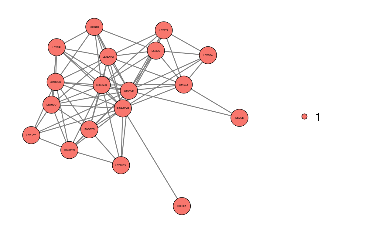
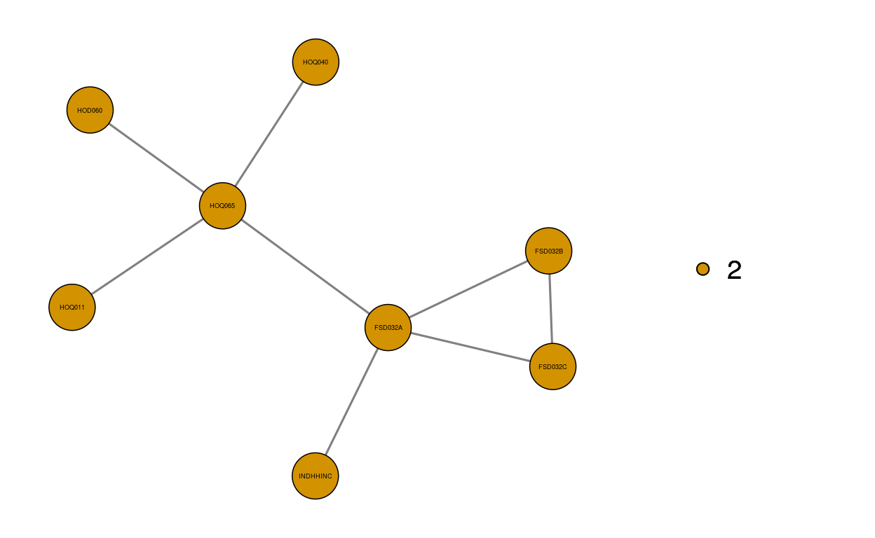
Using min_forest function we estimate the minimal forest with BIC method and detect communities in the graph. The first ten nodes with the highest betweenness centrality are shown. The estimated minimal forest and two of its communities are also illustrated.
mf <- min_forest(data, stat = "BIC", community = T, plot = F, levels = NULL)
mf$betweenness[1:10]
HUQ050 PAD200 PAQ100 PAQ180 HIQ011 RIAGENDR DIQ190B RIDRETH1
6264.000 5820.083 5508.500 5450.000 5450.000 5441.191 4858.167 4160.654
HUQ010 HSD010
3831.000 2799.000 mf$networkmf.val <- graph_vis(mf$graph, directed = F, community = T, betweenness = T, plot = T, plot.community = T, plot.community.list = c(1,2))
dim_reduce
In order to show the functionality of minimal forest in clustering, we select a subsample of size 200 and apply min_forest function (with parameter community = T) on the subsampled dataset. Therefore the transposed dataset is passed to the funciton.
t_nhanes <- as.data.frame(sapply(as.data.frame(t(data[1:200, ])), function(x) as.numeric(as.character(x))))
cluster_mf <- min_forest(t_nhanes, plot = T, community = T)
We use dim_reduce function with tsne and umap methods to reduce dimensionality of the aforementioned subpopulation. The points are colored according to their communities within the minimal forest.
 communities <- cluster_mf$communities
 communities <- communities[match(c(1:200), as.integer(names(communities)))]

## Using 'umap' method
 ump <- dim_reduce(data[1:200,], method = "umap", annot1 = as.factor(communities), annot1.name = "minimal forest\n communities")

## Using 'tsne' method
 tsn <- dim_reduce(data[1:200,], method = "tsne", annot1 = as.factor(communities), annot1.name = "minimal forest\n communities")

## Using cowplot to plot with shared legend
 require(cowplot)
 require(ggplot2)
 leg <- get_legend(ump + theme(legend.position = "bottom"))
 plt <- plot_grid(ump + theme(legend.position = "none"), tsn + theme(legend.position = "none"))
 plot_grid(plt, leg, ncol = 1, rel_heights = c(1, .2))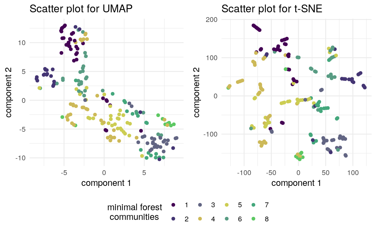
VKL
Focusing on the variable PAD590 (TV usage) we select two groups of samples: (i) The participants who watch TV less than an hour (g1) and (ii) those who watch more than 5 hours (g2) a day.
We calculate variable-wise Kullback-Leibler divergence between these two groups using VKL function (with permute = 100 to find p-values of the resulted variables).
g1 <- which(data$PAD590 == 1)
g2 <- which(data$PAD590 == 6)
KL <- VKL(data, group1 = g1, group2 = g2, permute = 100)
KL[2:6, ]
KL variable p.value
HSD010 0.2581593 HSD010 0.01
PAQ520 0.2193065 PAQ520 0.01
HUQ010 0.2157753 HUQ010 0.01
RIDAGEYR 0.2094270 RIDAGEYR 0.01
LBXALC 0.2066657 LBXALC 0.01VVKL
Using VVKL function with permute = 100, we find the most important (categorical) variables violating the linear relationship between LBXTC (total cholesterol) and LBXVIE (vitamin E). The result suggests DSD010 (taking dietary supplements) and DRQSPREP (type of table salt used) as variables with the highest KL-divergence.
KL <- VVKL(data[, 75:160], var1 = data$LBXTC, var2 = data$LBXVIE, plot = T, var1.name = 'LBXTC', var2.name = 'LBXVIE', permute = 100, levels = NULL)
kableExtra::kable(head(KL$kl, n = 5)) %>%
  kable_styling() %>%
scroll_box(width = "300px", height = "300px")| KL | variable | p.value | |
|---|---|---|---|
| DSD010 | 0.9975456 | DSD010 | 0.01 |
| RIDRETH1 | 0.1947663 | RIDRETH1 | 0.01 |
| PAQ520 | 0.1552019 | PAQ520 | 0.01 |
| HUQ050 | 0.1538361 | HUQ050 | 0.01 |
| HOD060 | 0.1436053 | HOD060 | 0.01 |
KL$plot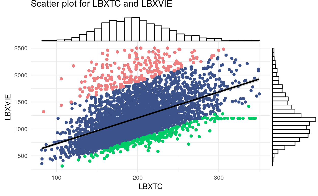
–>
plot_assoc
We use plot_assoc with levels = 15 to visualize a (pair of) variable(s) in the dataset.
Histogram of PAD600 (number of hours using computer last month. 0: less than hour, 1: one hour, …, 5: five hour, 6: None):
plot_assoc(data, vars = c("PAD600"), levels = 15, interactive = F)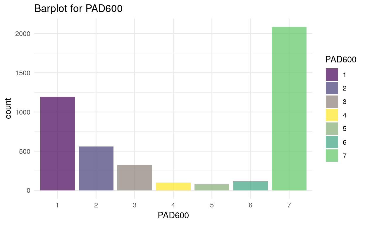
Density plot of RIDAGEYR (age):
plot_assoc(data, vars = c("RIDAGEYR"), levels = 15, interactive = F)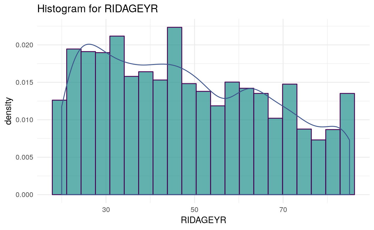
Boxplot of LBXTHG (total mercury amount in blood. ug/L) for different answers to DRD360 (fish eaten during past 30 days. 1: Yes, 2: No, 3: Refused, 4: Don’t know):
signif <- mf$significance
signif[signif$edges.from == 'DRD360' & signif$edges.to == 'LBXTHG', ]
edges.from edges.to statistics p.value
105 DRD360 LBXTHG 385.9683 1.574062e-05plot_assoc(data, vars = c("LBXTHG", "DRD360"), levels = 15, interactive = F)
Heatmap of DSD010 (taking any dietary supplements. 1: yes, 2: no, 3: refused, 4: don’t know) and SMD410 (smoking in the household 1: yes, 2: no):
signif[signif$edges.from == 'DSD010' & signif$edges.to == 'SMD410', ] edges.from edges.to statistics p.value
242 DSD010 SMD410 -101.8203 0.5359423plt <- plot_assoc(data, vars = c("DSD010", "SMD410"))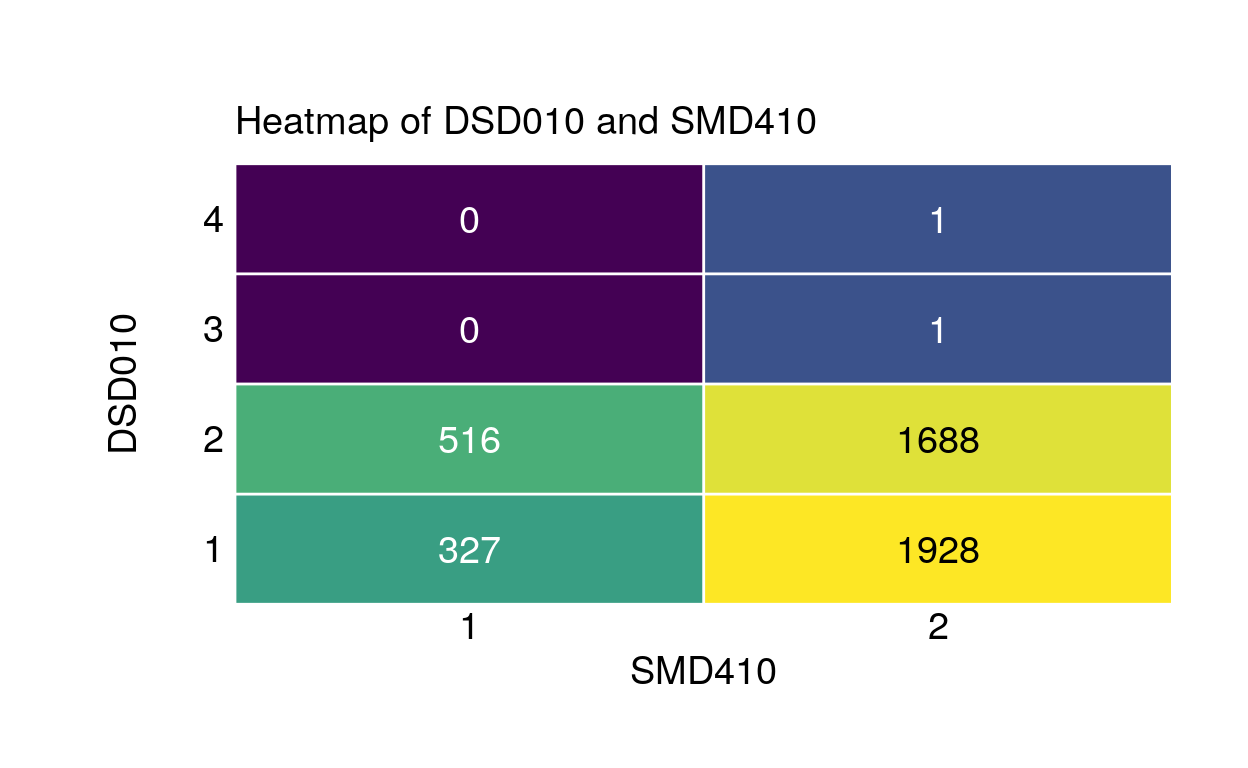
Scatter plot of LBXHGB (hemoglobin amount in blood. g/dL) and LBXSIR (refrigerated iron in blood. ug/dL):
signif[signif$edges.from == 'LBXHGB' & signif$edges.to == 'LBXSIR', ] edges.from edges.to statistics p.value
60 LBXHGB LBXSIR 802.3598 3.924962e-15plot_assoc(data, vars = c("LBXHGB", "LBXSIR"), levels = 15, interactive = F)